Manually tuning rewards to create human-like motion is an incredibly difficult task. I’ve spent the past few weeks going through some major works to better understand how you can use motion capture data to train policies that achieve human-like behavior. This blog covers only a small number of motion tracking papers. I hope to go over sim2real motion tracking efforts in a future blog post. In the meantime, I encourage you to do some searching on the latest works on training human-like motions using motion tracking!

DeepMimic: Example-Guided Deep Reinforcement Learning of Physics-Based Character Skills

DeepMimic is one of the most foundational papers behind motion tracking in simulation. Although the concept is pretty simple, there are a lot of neat tricks the authors do to improve performance in simulation.

Most RL policies trained in simulation are focused on ensuring that you maximize rewards while also ensuring that the reward aligns with the objective (ex. if you define the reward to make a robot walk, the robot learns to walk instead of exploiting the simulation to perform undesirable behavior). Reinforcement Learning in simulation can be sample inefficient; policies are vulnerable to unstable simulation physics or might perform actions that result in undesirable behavior (which you then use as data to further train the policy).

DeepMimic solves these problems by introducing a motion reference to RL policies. Instead of exploring the state space and rolling out episodes that don’t directly contribute to convergence, [1] introduces a framework where you can capture motion capture data of the desired task and use that data to “generate goal-directed and physically realistic behavior from those reference motions.”

The authors also define a phase variable $\phi \in [0, 1]$ that’s concatenated with the state features to denote progress along a motion (so $\phi = 0$ implies the beginning of a motion cycle and $\phi = 1$ denotes the end). For example, if I was teaching a policy to perform a backflip, I might define $\phi = 0$ to be when the robot is standing, $\phi = 0.5$ for when the robot is mid air, and $\phi = 1$ to be after the robot lands on the ground. You can assume for simplicity that assuming your frame length is length $T$, at some arbitrary timestep $t$, $\phi = \frac{t}{T}$ (which then gets wrapped around for cyclic episodes).

The idea is pretty straightforward: given some arbitrary goal $g_t$ and character state $s_t$, define some policy $\pi(a_t \vert s_t, g_t)$ to be the control policy, instead of defining just the task-specific reward $r^G(s_t,a_t,g_t)$, we also define an imitation reward $r^I(s_t,a_t)$, where the imitation reward encourages the policy’s behavior to align with the reference data. This means that we can define the reward at some timestep $t$ to be the following:

where $\omega^I, \omega^G$ represent the imitation and task weights respectively. Additionally, we define the reference motion to be $\hat q_t$, of which the actor is trying to imitate. We can expand the imitation reward to be defined as:

where $r_t^P$ is defined to be the pose reward, $r_t^v$ is the joint velocity reward between the actor and the reference motion, $r_t^e$ is the end-effector reward designed to encourage the policy to match the end-effectors (hand and feet) with the reference motion’s end-effector positions, and $r_t^c$ is the center of mass penalty, where we penalize the policy for drifting from the reference motion’s center of mass.

Formally, each component is defined as

Note that in the first term, $\ominus$ is defined to be the quaternion difference between the $j$-th joint angle between the reference motion and the policy, and $||q||$ denotes the scalar rotation of the quaternion around its axis. The weights for each imitation reward component are then defined as
$w^p = 0.65, w^v = 0.1, w^e = 0.15, w^c = 0.1$.

I think what was pretty interesting about the way the imitation rewards are defined is that they are all bounded to be between $[0, 1]$. Although the authors don’t provide an explicit reason as to why their reward is defined to be that way, I would assume it’s because capping the imitation reward at 1 allows for the policy to treat the imitation reward as a “signal” and not as an actual reward. This is especially important when you do domain randomization, as you want to mimic the behavior and not overfit the actions to the reference data.

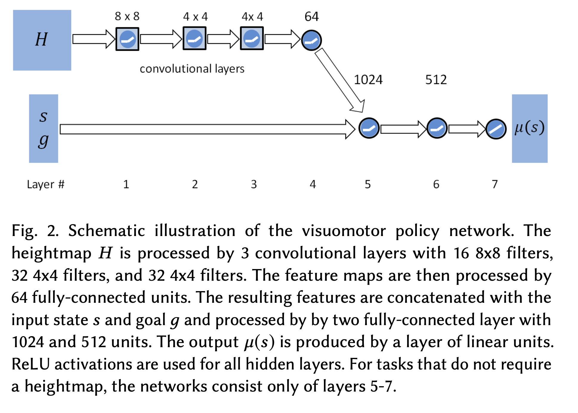
The actor is defined to be a feedforward neural network with 2 hidden layers of dims 1024 and 512. The action distribution space is defined as a Gaussian distribution, where the policy outputs the mean of these actions i.e. $\mu(s)$. This means that the action is sampled from a fixed covariance matrix, $a \sim \mathcal{N}(\mu(s), \Sigma), \ \ \pi(s) = \mu(s)$.

In the case where a heightmap is available, we instead define the actor as a visuomotor policy that encodes the image through convolution layers and then gets concatenated with state and goal information. This concatenated input space is then passed through the feedforward neural network.

Source: [1]

What if we wanted to learn multiple skills though? Instead of learning to just walk, what if we could learn to walk and perform a front flip? This would mean that we would use multiple motion reference clips to model our reward function, and prompt the user to determine what behavior we want. We can do this by defining the user-specified behavior as a one-hot vector where each index corresponds to a different behavior in our motion reference database, and pass this vector into the action policy. Also, instead of having to retrain new policies for every possible motion, you can instead train a policy for each unique motion in your dataset (yielding $k$ policies). At runtime, you can then use the value functions from each learned policy to determine what policy should be executing motion.

Our composite imitation reward would instead be defined to be the max reward of all the possible individual imitation rewards:

In this case, we do not have a task objective reward $r_t^G$ since we are optimizing to match the multi-goal imitation references (these independent policies are already trained with respect to their individual task-specific reward and imitation references). So in a sense, you can think of this as a Mixture of Experts (MoE) for actor networks (the authors formally call it MCAE, mixture of actor-critics experts model).

In order to determine what policy to roll out at every time frame, DeepMimic uses a Boltzmann distribution to model their composite policy:

note that $\mathcal{T}$ is defined to be the temperature parameter, where a higher temperature would indicate a more uniform probability across all policies and the opposite for lower temperature.

DeepMimic uses 2 main tricks in order to generate smooth motions that can be deployable in the real world: they randomize the initial state distribution along with implementing early termination of episodes.

Randomizing the initial state distribution means that instead of $\phi=0$ at the beginning of each episode, we can instead begin episodes in the middle of a reference motion. For example, if you wanted to train a policy to learn how to do a cartwheel, instead of starting the robot upright at the beginning of an episode, you might initialize the position so that the robot has its hands on the ground (handstand). This would aid exploration, allowing for the policy to realize that being in a handstand gives you a high reward compared to simply standing upright and moving your hands. Formally, the authors define this strategy as reference state initialization (RSI).

Early termination basically allows you to terminate and restart an episode if certain conditions were met. For example, if I was a robot trying to learn how to walk, I might define an early termination to be when the head or torso of the robot hits the ground. This is because once the robot hits the ground, it will be unable to physically walk, so the episode rollouts we collect from those states don’t help train our policies at all (you can think of these as garbage states). By terminating early, we’re able to improve the sample efficiency of the actor-critic networks (meaning that the observations we’re passing in increase robustness instead of rolling out garbage episode rollouts), allowing for a better generalist policy.

In a sense, you can think of both of these tricks as ways to increase the sample efficiency of the RL policy. Training RL policies often require significant reward tuning in order to ensure that the policy’s behavior aligns with the user’s goal. Through episode randomization techniques and early termination, the authors are able to pass higher quality data into the actor and critic networks, allowing for them to learn what good and bad behavior would look like.

Source: [1]. Notice how there's different possible starting joint positions we can initialize the robot to be in.

I won’t go over how the authors train their actor-critic network but they use the standard PPO actor-critic setup. The value function is computed with multi-step TD-$\lambda$ and the advantage function is learned using GAE. If you’re unfamiliar with these terms, check out my other blog post going over RL algorithms!

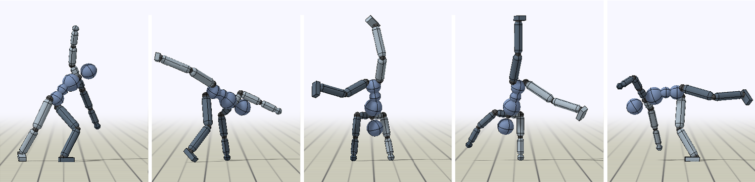
Here’s the video from the authors going over their results and methods:

These motions look great! I think one of the coolest things about this work was the ablation studies they did at the end, showing how crucial early termination is for skill reproduction. For more dynamic skills, the RSI method they proposed significantly helps as well. My guess is that early termination allows for better sample efficiency, while RSI can aid in the exploration process at the beginning (since starting in different joint positions can allow the policy to see what possible joint states give high and low rewards, which is especially useful in high dimensional spaces).

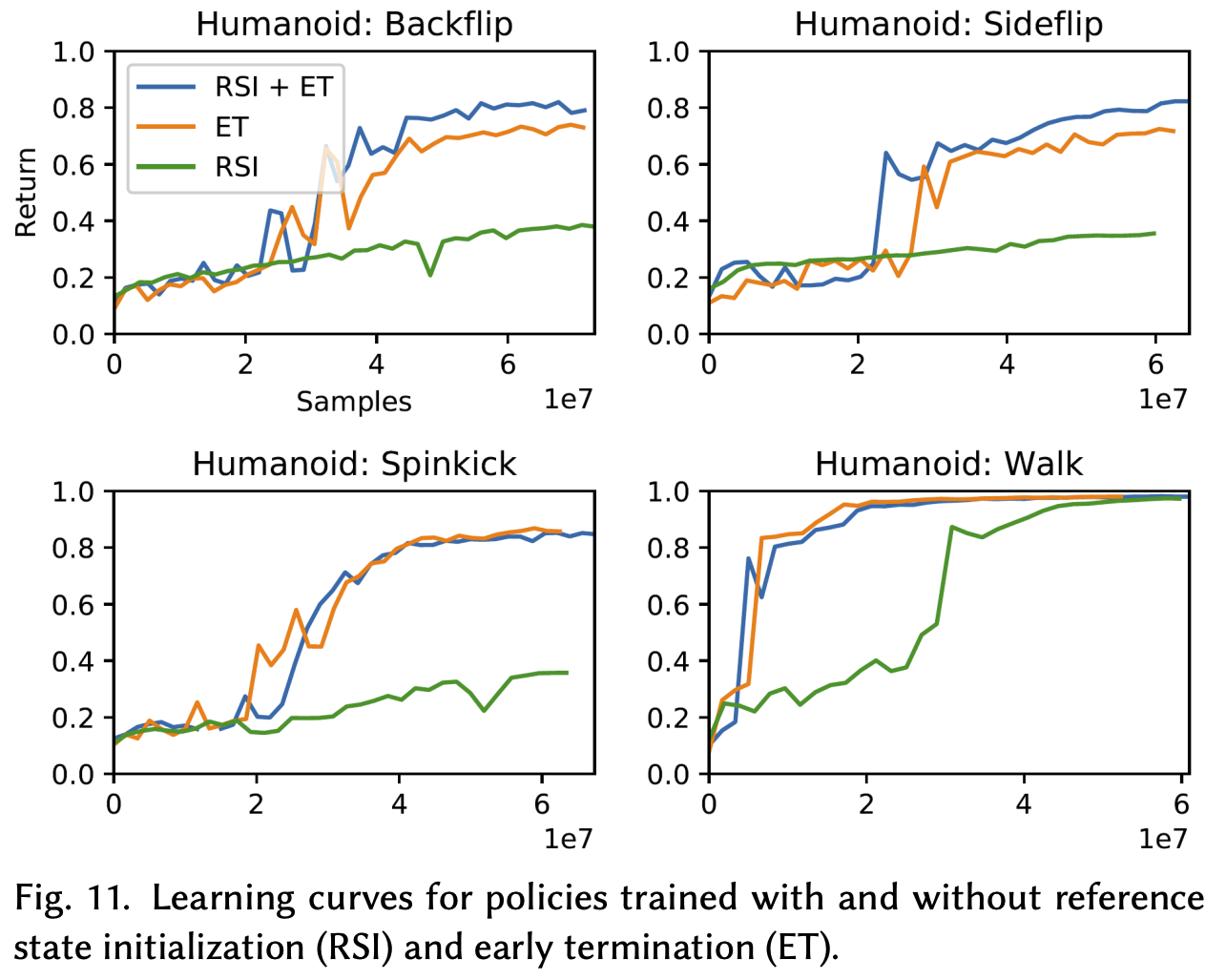
Source: [1]

AMP: Adversarial Motion Priors for Stylized Physics-Based Character Control

AMP [2] is a follow up to DeepMimic where the authors propose an even more general motion imitation pipeline to perform multiple tasks. In DeepMimic, we define objective functions for multi-skill control i.e. if I wanted to learn how to run and then perform a flip, I would have to manually determine the point in the episode where I might switch my imitation objective from running motion data and then frontflip motion data (which would then also tune our phase variable, $\phi$). side note: I hope it’s obvious why that $\phi$ doesn’t scale as we collect more and more data.

AMP alleviates the need for carefully tuned imitation objectives. Instead, we can use the goal reward to help define the objective of the policy (high-level control) while the execution (low-level control) of the policy can be defined from a dataset of “unstructured motion clips.” What this essentially means is that instead of having to manually pull out running or frontflip motion data to train the policy, you can simply pass in the entire motion dataset, which you use to train an “adversarial motion prior.” It is this prior that you train that helps define the style reward of the policy execution, allowing for human-like motion while performing the task.

You can think of this Adversarial Motion Prior as the discriminator network of a Generative Adversarial Network (GAN) [4], where you’re differentiating between actions and joint states of the policy and the dataset. To reiterate: instead of having to directly define the imitation objective and perform some form of imitation loss (like L2 loss) against the motion data, we instead define a network that learns the “realism” of our motions, which we then use to help train a policy that performs realistic motions (i.e. would be in distribution of our motion data).

One of the other issues with using an imitation loss with respect to motion data is that because you define pose errors between the joint angles of the robot and the reference data, it’s hard to define an objective imitation loss with respect to all skills that you’re trying to learn. In cases of where you might perform domain randomization, the motion capture data that you collect might not be in reference to the simulator (because the physics parameters that your dataset is collected in can possibly be out of distribution of the agent). By training an adversarial discriminator to differentiate between the motion dataset and the policy actions, you can create an objective function to train a policy to follow in-line with the demonstrations.

We define this method of training an adversarial discriminator as Generative Adversarial Imitation Learning (GAIL) [3]. We define the GAIL objective to be the following: given some dataset of states and actions $\mathcal{D} = \{(s_i, a_i)\}$, we train some discriminator $D(s, a)$ to predict whether a given state and action is sampled from $\mathcal{D}$ or from the policy $\pi$, where we define the objective to be the following:

where $d^\mathcal{M}$ is defined to state-action distribution of the motion capture dataset and $d^\pi$ is defined to state-action distribution of the actor policy network. One of the issues with this definition is that looking at state-action pairs would result in us capturing motion kinematic data and comparing our actions from the dataset to the policy, which is not what we want. Another situation might be where we are only given states of the motion reference clips (and not the action from that state). Instead, we can compare two consecutive states so that the discriminator can learn a form of the transition dynamics between 2 states of the joint positions of the robot to determine what would be “realistic” motion.

Standard GANs [4] deal with mode collapse and vanishing gradients because of the sigmoid cross-entropy loss. We can instead use the Least-Squares GAN (LS-GAN) [5] and add a gradient penalty, where the discriminator predicts the score of $1$ for samples from the dataset and $-1$ for samples from the policy. We then define the updated objective to be the following:

The authors note that passing in state transition information (the dynamics between the two states) can help the discriminator with more effective feedback. Between the two observation state frames, the authors pass in the following additional information:

• linear + angular velocities of the root
• local rotation + velocities of each joint
• 3-D positions of the end-effectors i.e. hands + feet

They define this additional information as an observation map $(\Phi(s), \Phi(s'))$ which is what gets passed into the discriminator $D$.

Once we train this discriminator, we use it to train the policy with Reinforcement Learning, where the policy reward is defined by:

Just like the standard GAN [4], the goal here is to be able to create a policy whose state-action distribution is indistinguishable from the dataset (from the perspective of the discriminator). This helps us define the overall task reward to be both the imitation reward and the goal objective reward:

where $r^G$ is the task-specific reward and $r^S$ is the style (imitation) reward. Similar to DeepMimic [1], the authors use the standard PPO actor-critic setup. The value function is computed with multi-step TD-$\lambda$ and the advantage function is learned using GAE. The actor is modelled to return a Gaussian distribution over actions $\pi(a_t \vert s_t, g) = \mathcal{N}(\mu(s_t, g), \Sigma)$ where $\Sigma$ is the covariance matrix and is manually specified and kept fixed. Our training loop would look like this:

1. define $\mathcal{M}$ to be the dataset of reference motions, $D$ to be the discriminator, $\pi$ to be the actor policy, $V$ as the value function, and $\mathcal{B} = \emptyset$ to be the replay buffer.
2. while policies not converged:
   1. for trajectory $i=1, .., m$:
      1. collect trajectory $\tau^i = \{(s_t, a_t, r_t^G)_t=0^{T-1}, s_T^G, g\}$ by rolling out $\pi$.
      2. for each timestep $t = 0,..., T$:
         1. predict motion similarity $d_t = D(\Phi(s_t), \Phi(s_{t+1}))$.
         2. calculate style reward $r(s_t, s_{t+1}) = \max \left[0, 1-0.25(d_t-1)^2 \right]$.
         3. calculate total reward $r_t = w^G r^G + w^S r^S$.
         4. record $r_t$ in $\tau^i$.
      3. store $\tau^i$ in $\mathcal{B}$.
   2. for each update step $1, ..., n$:
      1. sample $K$ transitions $\{(s_j, s'_j)\}_{j=1}^K$ from $\mathcal{M}$.
      2. sample $K$ transitions $\{(s_j, s'_j)\}_{j=1}^K$ from $\mathcal{B}$.
      3. update discriminator params $D_\theta \leftarrow D_\theta - \alpha \nabla_\theta L_D$ where
         $$L_D = \frac{1}{K}\sum_{j=1}^K \left[(D_\theta(\Phi(s_j^\mathcal{M}), \Phi(s_j'^{\mathcal{M}}))-1)^2 + (D_\theta(\Phi(s_j^\pi), \Phi(s_j'^{\pi}))+1)^2 + \frac{w^{\text{gp}}}{2}\left\|\nabla_\phi D_\theta(\phi)\big|_{\phi=(\Phi(s_j^\mathcal{M}),\Phi(s_j'^{\mathcal{M}}))}\right\|^2\right]$$
   3. update $\pi$ and $V$ according to trajectory data $\{\tau^i\}_{i=1}^m$.

For tasks, the authors set $w^G=0.5$ and $w^S=0.5$, and $w^{\text{gp}} = 10$. Their ablation studies are pretty interesting as well; they show that without the gradient penalty, large performance fluctuations are evident throughout training. This is also noticed in other experiments where they remove velocity information into the discriminator in tasks (like the rolling task) where the policy doesn’t seem to converge. This could possibly be because velocity information is crucial in dynamic tasks for the discriminator to differentiate realistic behavior.

What’s cool about these results is that these motion prior policies seem to do as well as the motion tracking policies without ever defining an explicit imitation reward. This shows that it is indeed possible to train a policy with good style without ever having to manually define a motion imitation reward!

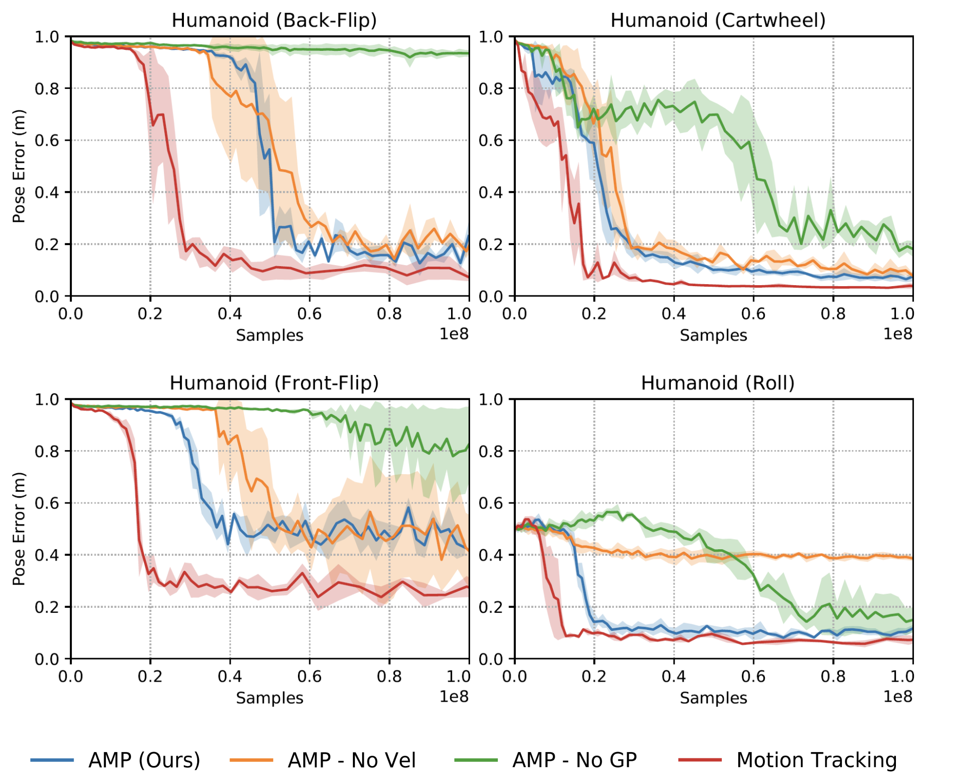
Source: [2]

InterMimic: Towards Universal Whole-Body Control for Physics-Based Human-Object Interactions

InterMimic builds on the idea of motion references for human object interactions (HOI). The idea here is pretty straightforward: leverage existing motion capture (MoCap) datasets and retarget them onto the robot (UniTree G1 with inspire hands) in sim. Then, train separate teacher policies for multiple tasks and distill them into a student policy that can perform multiple tasks. After, finetune the student policy with Reinforcement Learning to create a policy that can perform multiple tasks!

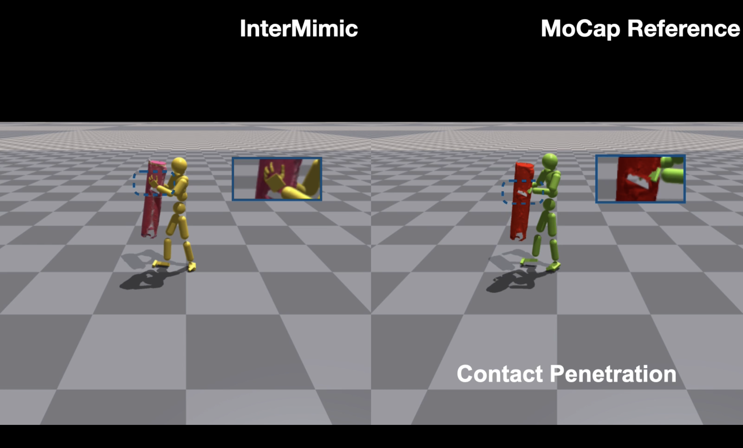
MoCap data in general is really good at providing references to train policies with (as we saw in the DeepMimic works). There are two main issues with using MoCap data for human object interactions: 1) your reference data might be coming from a different robot (resulting in hardware differences) and 2) replaying reference data in simulation can result in unstable dynamics. We can solve 1) with motion retargeting while preserving interaction dynamics but 2) is a pretty unsolved problem.

Source: [6]

The idea here is to essentially start by loading in the reference motions in simulation (just like how we loaded motion references in simulation in the DeepMimic paper), which the authors call Reference State Initialization (RSI). The issue with blindly loading in reference data is that you introduce “critical artifacts,” such as object penetration and unrecoverable failures (like dropping an object). What InterMimic proposes instead is an initialization method known as Physical State Initialization (PSI). Instead of using all the reference initialization data we’re given, we should instead try to sample quality references initializations with higher probability.

The authors go about this by creating an initialization buffer to store MoCap + simulation states. Then, for every rollout in simulation, randomly sample an initial state from the buffer. This can allow for the policy to observe more advantageous states. At the end of an episode, trajectories are then evaluated with respect to their expected discounted rewards. If the expected discounted reward exceeds some threshold (that they manually define), the trajectory is added to the buffer in a queue-like (FIFO) style. Once this buffer is filled up, older/lower-quality trajectories will be thrown out in place for higher expected discounted rewards.

One thing to note here is that there is a very real chance that the state at $t=0$ isn’t advantageous for the policy at all when it rolls out with respect to the MoCap data. For example, if my task was to pick up a cube on the table, my buffer might contain states where the robot’s hand is very close to the cube or the cube gets picked up by the policy and is in the air. The motivation behind this idea is that “learning later-phase motion can be essential for policies to achieve high rewards during earlier phases, compared to incrementally learning from the starting phase.” I think this statement does make sense; learning later-phase movement allows the policy to see states with high rewards, allowing for an implicit understanding of “desired goal states” that it would act on at environment initialization.

The goal of human object interaction is to create some motion $\{q_t\}_{t=1}^T$ to match the reference MoCap data $\{\hat{q_t}\}_{t=1}^T$, where $q_t = \{q_t^h, q_t^o\}$, which represent the human pose and the object pose. $q_t^h = \{\theta_t^h, p_t^h \}$ where $\theta_t^h \in \mathbb{R}^{51 \times 3}$ is defined to be the joint rotations and $p_t^h \in \mathbb{R}^{51 \times 3}$ is defined to be the joint positions. The robot in simulation is 51-dof, with the hand having 30 joints and the body having 21 joints. $q_t^o = \{\theta_t^o, p_t^o \}$ where $\theta_t^o \in \mathbb{R}^{3}$ is defined to be the object orientation and $p_t^o \in \mathbb{R}^{3}$ is defined to be the object position.

The inputs to the actor policy are the following: $s_t = \{s_t^s, s_t^g\}$, where

which consists of the human + object joint angles, positions, angular velocities, and linear velocities along with the vector from the human joint to their nearest point on object surface ($d_t$) and a binary contact marker ($c_t$) to indicate contact on the body of the robot.

$s_t^g$ is defined to be reference differences in poses between the current pose and the motion reference pose at $k \in \mathcal{K}$ timesteps in the future. This is formally defined as

where $\hat{\theta}_{t+k}^h, \hat{p}_{t+k}^h, \hat{d}_{t+k}, \hat{c}_{t+k}$ is the motion reference information at time step $t + k$. For example, if $\mathcal{K} = \{1,2,3\}$, at some arbitrary timestep $t$, we would take the relative pose differences of the joint angles, positions, human-to-object surface vectors, and contact markers at timesteps $t+1, t+2, t+3$.

The policy is defined as an MLP with dimensions [1024, 1024, 512]. The action space is defined as $a_t \in \mathbb{R}^{51 \times 3}$, since the robot has 51 joints. This is essentially joint space control but the key distinction that we’re doing joint space control with respect to the 3 (x,y,z) axes. This is why our action space is in the $51 \times 3 = 153$ dimensions.

To recap, the teacher policy we’re training is not trained as an imitation objective between the teacher and the motion reference data. Instead, what we are doing is defining “style rewards” in the form of embodiment-aware and embodiment-agnostic rewards. We define embodiment-aware to be the rewards concerning with the joint angles and position differences between the referenced motion and the human motion. The goal here is that when the robot is far away from the object, our motion retargeting should specifically focus on ensuring that the rotational motion of the joints line up with the referenced motion and when the robot is close to the object, retargeting with respect to position is important for stable contact.

My understanding of the idea here is that when the robot is far away from the object, prioritizing rotational motion will ensure that you capture the movement pattern between different bodies. Because the reference data does not necessarily use the same robot body as the policy that we’re training, using position-based penalties when the object is far away wouldn’t take into account the physical differences (ex. longer limbs or arms), which makes rotation-based reward a better reward model. And once you’re close to the object, you want to take smaller steps for fine-grained manipulation, which is why position tracking becomes important. The authors define this to be modelled as the following:

where $\langle \cdot, \cdot \rangle$ is defined to be the inner product. We also define $\Delta_p^h[i] = ||\hat{p}^h[i] - p^h[i]||$ to be the position delta between the reference motion and the robot end-effectors, $\Delta_\theta^h[i] = ||\hat{\theta}^h[i] \ominus \theta^h[i]||$ to be the rotational difference, and $\Delta_d[i] = ||\hat{d}[i] - d[i]||$ to be the contact directional vector displacements. The weight $w_d$ is meant to be inversely proportional to the distances between the joints of the robot and the object. So, for example, if $w_d = 0$, then we would care about the rotational difference and not the position difference since we would be far from the object, while the opposite would occur when the robot is close to the object.

The authors define the weight $w_d$ to be the following:

What we’re basically doing here is defining the weight to be the average normalized distance between the robot joint to the object for both the robot joints and the reference motion joints. Why model everything as an exponential? Because joints closer to the object should have a higher weight (ex. hands and fingers), so we should care much more about the positions of these end-effectors compared to their joint angles. But for joints like legs and the head, we might care more about the rotational difference since their positions don’t really matter as much.

The reward objective for each of these cost functions ($E_p^h, E_\theta^h, E_d$) can be defined to be the maximum of $\exp{(-\lambda E)}$, where $\lambda$ is an arbitrary hyperparameter (sharpness).

The embodiment agnostic reward takes into account the information needed for object tracking and contact tracking, where object tracking cost is defined as $E_p^o = ||\hat{p}^o - p^o||$ and rotation $E_\theta^o = ||\hat{\theta}^o - \theta^o||$. We also define a contact reward to ensure that the right joints are making contact with the object, which are broken down into a contact promotion reward $E_b^c$ and a contact penalty $E_p^c$. We define these to be the following:

There are 3 levels to contact rewards: promotion, penalty, and neutral. This is to help the policy “accommodate potential inaccuracies in reference contact distances.” To also ensure that the policy learns to perform accurate manipulation, a hand contact guidance reward is introduced. Because a lot of the reference data uses flattened hand poses, activating reference contact markers when the hand is near the object allows for the policy to learn human interaction strategies. This contact reward is modelled as the following:

where $\hat{c}^{\text{lhand}}, \hat{c}^{\text{rhand}}$ are defined when the hand is below some distance threshold $\sigma$ to the object.

Putting this all together, we get the overall following reward function for the teacher policies:

where $E_h^e = \sum ||a_h||$, $E_o^e = \sum ||a_o||$, and $E_c^e = \max ||f||$ are energy costs of the joints, object’s acceleration, and forces respectively.

The teacher policy is trained using the standard PPO algorithm where advantage estimates are given by $\text{GAE}(\lambda)$. The authors also use early termination conditions such as:

• when object points deviate from the reference by >0.5 m
• weighted average distances between the robot’s joints and the object >0.5 m
• contact that should occur doesn’t for more than 10 consecutive frames

Once we train our teacher policies, we chain these teachers together to train the student policy that’s capable of “mastering” all skills via distillation. The authors start with DAgger [7] and then finetune the policy with RL (PPO). By doing this, you’re able to have the student policy be as good as the teacher policies (since we are taking a supervised objective with respect to the teacher), and then rolling out the student policy with RL in simulation allows for the possibility for the student policies to be better than the teacher policies.

Another thing to also note is that when we train the teacher policies, notice in the state observations that we take the relative differences with respect to the mocap data. For the student policies though, we define $s^S$ to use the teacher states as the ‘reference’ states (instead of the mocap), since the mocap data is noisy and imperfect (which is fixed by the teacher).

The overall distillation + RL algorithm can be defined as the following:

1. Define H to be the PPO horizon length, student policy parameters $\psi$, student value function parameters $\phi$, and some ‘composite’ policy $\pi^{(T)}$ to be all the chained teacher policies.
2. for iterations $t = 0, 1, 2, \ldots$:
   1. for $h$ from $1... H$:
      1. sample $u \sim \text{Uniform}(0, 1)$
      2. step $s^{(T)}, a^{(T)}$ from teachers $\pi^{(T)}$
      3. define the references in $s^{(S)}$ to use the teacher policy $s^{(T)}$
      4. define the student action $a^{(S)}$ to be from the student policy $\pi_{\psi}^{(S)}(a^{(S)}|s^{(S)})$
      5. if $u \leq \frac{t}{\beta}$ then (step with the student)
         1. step with $a^{(S)}$ in the simulator, observe $s'^{(S)}, r$
      6. else (step with the teacher)
         1. step with $a^{(T)}$ in the simulator, observe $s'^{(S)}, r$
      7. Store the transition $(s^{(S)}, s'^{(S)}, a^{(S)}, a^{(T)}, r)$
   2. update value function parameters $V_\phi$ with $\text{TD}(\lambda)$ algorithm
   3. compute PPO objective: $L(\psi)$
   4. compute imitation loss $J(\psi) = ||a^{(S)} - a^{(T)}||$
   5. compute the weight: $w = \min(\frac{t}{\beta}, 1)$
   6. update student policy parameters $\psi \leftarrow \psi - \alpha \nabla_{\psi}(wL(\psi) + (1-w)J(\psi))$

Using this BC-RL finetuning loop shows some pretty promising results!

ADD: Physics-Based Motion Imitation with Adversarial Differential Discriminators

One of the bigger issues with the DeepMimic and AMP works was that you still had to manually reward tune each parameter to get optimal performance. What ADD [8] introduces instead is a “novel adversarial multi-objective optimization (MOO) technique” where you replace the traditional reward structure (which outputs a scalar) with a “vector of objective values.” The values in this vector might be defined as the difference between the ideal performance (or motion capture data), and the current performances of a model.

For example, a differential vector $\Delta_t$ for motion tracking might be defined as:

where $p_t^I, v_t^I, e_t^I$ represent the reference pose, velocity, and end-effector positions from the motion capture data, and $p_t, v_t, e_t$ are from the robot (policy) in simulation. In the ADD paper, $\Delta_t$ is defined as the “negative relative difference” between the reference data and the policy, which would be $0 - (p_t^I - p_t)$ instead of just $p_t^I - p_t$. By doing this, you guarantee that the only positive vector you get will be when the policy perfectly matches the motion reference data (which would mean that you get the zero vector).

Using this information, we can then create an adversarial differential discriminator to take in this vector of relative differences (you can also interpret this vector as an error vector) and output a value between 0 and 1 representing how close the current motion is to perfect (compared to how ‘realistic’ the motion was in AMP). The reason why the authors define the discriminator to be like this is because even if the errors for some objectives (such as velocities) are zero, if the pose error is high, this might imply that the policy is not correctly matching the ideal positions, resulting in suboptimal performance.

This allows us to define the Multi-objective optimization problem as a mini-max game, since we know that $\mathcal{D}(\mathbf{0}) = 1$:

As I mentioned previously, one of the key differences between ADD and prior adversarial learning frameworks (AMP) is that the discriminator only sees one ‘ideal’ example (the zero vector, $\Delta = \mathbf{0}$), which the authors find to work well in training. To ensure that the discriminator properly learns to assign good scores, the authors also add the same gradient penalty idea introduced in AMP:

Similar to DeepMimic, the observation map contains the following set of features:

• Global position and rotation of the root
• Position of each joint represented in the character’s local coordinate frame
• Global rotation of each joint
• Linear and angular velocity of the root represented in the character’s local coordinate frame
• Local velocity of each joint

We then define $\Delta_t$ to be the difference between the reference data and the policy i.e.
$\Delta_t = \phi(\hat{s}_t) \ominus \phi(s_t)$.

We also define the reward to simply be a singular term, based on the output of the discriminator:

Just like in previous works, training follows an actor-critic setting where the policy is trained with PPO. Advantages are computed with GAE($\lambda$), and the value function is updated using the TD-$\lambda$ algorithm. The training loop can be a little confusing but the important thing to note here is that the discriminator is trained as the actor and critic networks are trained as well, there is no form of pre-training here!

You can define the overall training loop to be as follows:

1. Define $\mathcal{M}$ to be the reference motion clip dataset, $\mathcal{D}$ as the discriminator, $\pi$ as the actor policy network, value function $\mathcal{V}$, $\mathcal{B} = \emptyset$ as the experience buffer, mini-epochs $n$, and episode length $T$.
2. while not done, do:
   1. for trajectory $1, ..., m$ do:
      1. collect episode trajectory $\tau^i = \{(s_t, a_t)_{t=0}^{T-1}, s_T\}$ by rolling out $\pi$
      2. collect reference episode trajectory $\tau^i = \{(\hat{s}_t)_{t=0}^{T-1}\}$ from $\mathcal{M}$
      3. for $t =0, ..., T-1$:
         1. update $\Delta_t = \phi(\hat{s}_t) \ominus \phi(s_t)$
         2. compute discriminator output $d_t = \mathcal{D}(\Delta_t)$
         3. calculate reward $r_t = -\log(1 - d_t)$
         4. store $r_t$ in $\tau^i$
      4. store $\tau^i$ in $\mathcal{B}$
   2. for mini-epochs $1, ..., n$:
      1. for each batch $b^\pi$ from $\mathcal{B}$:
         1. update $\mathcal{D}$ using the definitions above
         2. update $\mathcal{V}$ using TD-$\lambda$
         3. update $\pi$ using PPO surrogate objective and GAE($\lambda$)

And the results seem pretty cool!

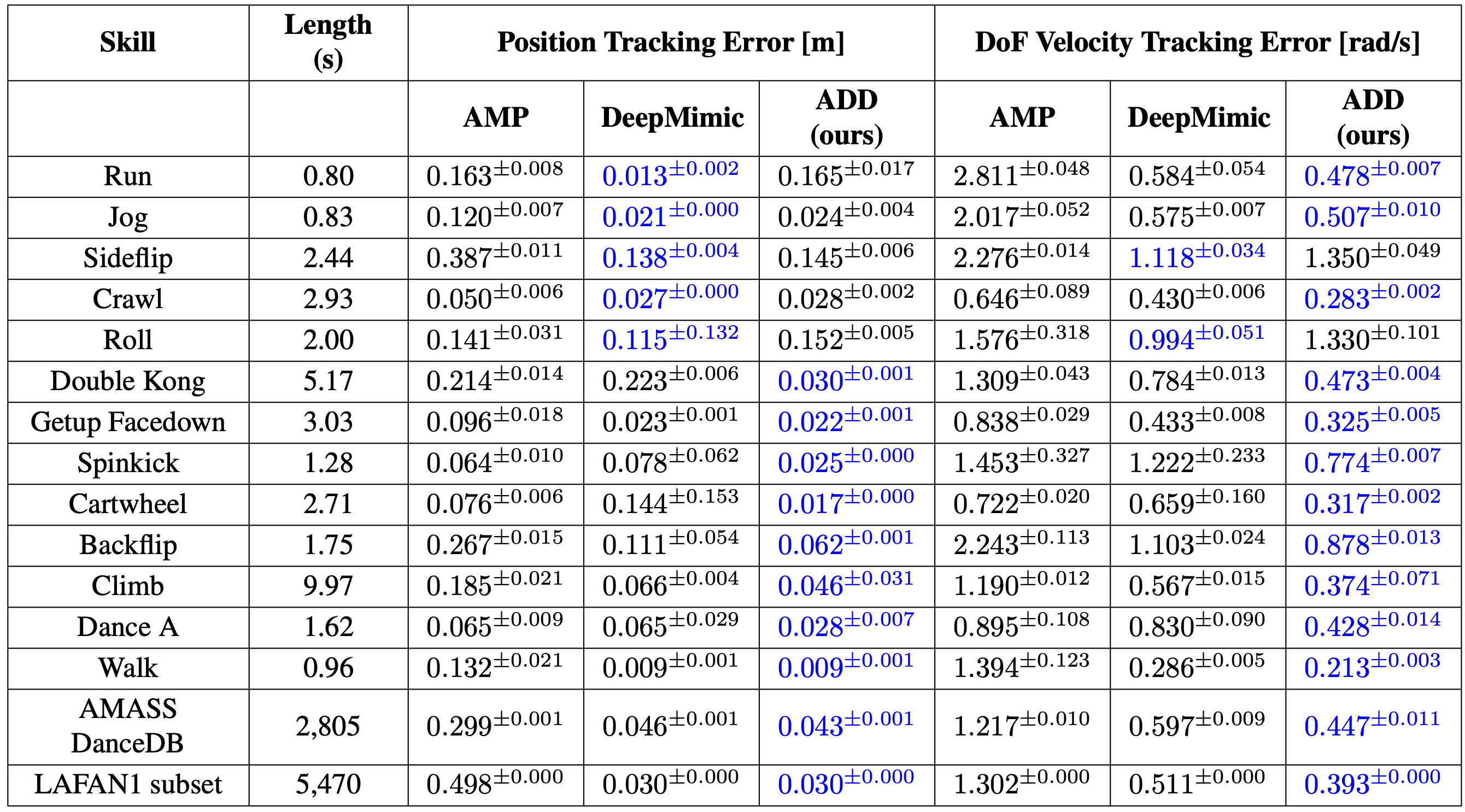
The authors do lots of comparisons to previous frameworks (DeepMimic, AMP) to see how well ADD performs. Here’s an image of their table comparisons:

Source: [8]

I think the main takeaway here is that ADD is pretty powerful in performing more diverse and difficult motions, while DeepMimic still shows really good performance in simpler motions (like running and rolling). What the authors note is that “ADD is less precise than DeepMimic on some forward locomotion skills, such as humanoid running and robot walking. The performance gap stems from ADD’s difficulty in accurately tracking the root position, which is crucial for imitating forward locomotion behaviors.”

Additionally, “the gradient penalty restricts the discriminator from assigning significantly larger weights to the root position errors.” This essentially means that if we cared much more about root position errors than other metrics (such as velocity), the gradient penalty doesn’t incentivize the discriminator to “care” more about the root position errors. Although there is no form of reward tuning done with ADD, in a way you might possibly have to do some form of “differential vector tuning” for stable convergence ;)

One of the main takeaways I had reading through some of these motion tracking works is that DeepMimic, although simple, is a very powerful framework to learn to imitate “human-like motions.” Adversarial-based learning techniques like AMP and ADD scale this work help build on this idea of “human-like motions,” but there is a lot of work to be done in training these discriminators since GANs are pretty unstable. The nice thing about the idea of ADD is that you don’t have to manually tune rewards, which is very convenient for training RL policies in simulation.

Thank you to Andrew Wang for our discussions about the papers in this blog. The chance that there is a mistake that I haven’t caught yet is pretty high 😅. If you do find one, whether it’s a typo or a mistake in an explanation, contact me at srianumakonda@cmu.edu!

Citation

If you found this blog post helpful, you can cite it as:

@article{anumakonda2025motiontracking,
  title   = {Motion Tracking Notes},
  author  = {Anumakonda, Sri},
  journal = {srianumakonda.github.io},
  year    = {2025},
  month   = {November},
  url     = {https://srianumakonda.github.io/posts/motiontracking/}
}

References

1. Peng, X. B., Abbeel, P., Levine, S., & van de Panne, M. (2018). DeepMimic: Example-guided Deep Reinforcement Learning of Physics-based Character Skills. ACM Transactions on Graphics, 37(4), 143:1–143:14. https://arxiv.org/abs/1804.02717
2. Peng, X. B., Ma, Z., Abbeel, P., Levine, S., & Kanazawa, A. (2021). AMP: Adversarial Motion Priors for Stylized Physics-Based Character Control. ACM Transactions on Graphics, 40(4), 1-20. https://arxiv.org/abs/2104.02180
3. Ho, J., & Ermon, S. (2016). Generative Adversarial Imitation Learning. Advances in Neural Information Processing Systems, 29. https://arxiv.org/abs/1606.03476
4. Goodfellow, I. J., Pouget-Abadie, J., Mirza, M., Xu, B., Warde-Farley, D., Ozair, S., Courville, A., & Bengio, Y. (2014). Generative Adversarial Networks. Advances in Neural Information Processing Systems, 27. https://arxiv.org/abs/1406.2661
5. Mao, X., Li, Q., Xie, H., Lau, R. Y. K., Wang, Z., & Smolley, S. P. (2017). Least Squares Generative Adversarial Networks. Proceedings of the IEEE International Conference on Computer Vision (ICCV). https://arxiv.org/abs/1611.04076
6. Xu, S., Ling, H. Y., Wang, Y.-X., & Gui, L. (2025). InterMimic: Towards Universal Whole-Body Control for Physics-Based Human-Object Interactions. Proceedings of the IEEE/CVF Conference on Computer Vision and Pattern Recognition (CVPR). https://arxiv.org/abs/2502.20390
7. Ross, S., Gordon, G., & Bagnell, D. (2011). A Reduction of Imitation Learning and Structured Prediction to No-Regret Online Learning. Proceedings of the Fourteenth International Conference on Artificial Intelligence and Statistics, 15, 627-635. https://arxiv.org/abs/1011.0686
8. Zhang, Z., Bashkirov, S., Yang, D., Shi, Y., Taylor, M., & Peng, X. B. (2025). Physics-Based Motion Imitation with Adversarial Differential Discriminators. SIGGRAPH Asia 2025 Conference Papers. https://arxiv.org/abs/2505.04961